EEG Bandpower

Electroencephalography (EEG) measures electrical activity in the brain using electrodes placed on the scalp. EEG signals provide insights into brain function and are used in various applications, including clinical diagnosis, neuroscience research, and brain-computer interfacing. A critical aspect of EEG analysis is the extraction of different band powers from EEG data and the computation of spectral density. This article explores the methodologies for extracting band powers from EEG data and computing spectral density, highlighting their importance and applications. This project deals with the extraction of data from an EEG, the separation of its constituent bands, and the calculation of their respective band powers

Types of Bands

EEG signals are typically decomposed into different frequency bands, each associated with distinct neural processes:

1. Delta (0.5-4 Hz): Dominant during deep sleep and in pathological conditions such as brain injuries.
2. Theta (4-8 Hz): Related to drowsiness, light sleep, and certain cognitive tasks such as memory encoding.
3. Alpha (8-13 Hz): Associated with relaxed wakefulness and is most prominent in the posterior regions of the brain when the eyes are closed.
4. Beta (13-30 Hz): Linked to active thinking, concentration, and motor activity.
5. Gamma (30-100 Hz): Associated with high-level cognitive functions, including perception and consciousness.

Methods for Bandpower Extraction

1. Fourier Transform

The Fourier Transform (FT) is a mathematical technique that converts a time-domain signal into its constituent frequencies. In EEG analysis, the Discrete Fourier Transform (DFT) or its efficient computation, the Fast Fourier Transform (FFT), is commonly used to obtain the power spectral density (PSD) of the signal.

a. Preprocessing

EEG data is often preprocessed to remove artifacts such as eye blinks and muscle movements. Common preprocessing steps include filtering, segmentation, and artifact rejection.

b. Windowing

EEG data is typically divided into overlapping segments or windows to enhance the frequency resolution and reduce spectral leakage.

c. FFT Computation

The FFT is applied to each windowed segment to compute the PSD. The PSD is then averaged over all segments to obtain the overall PSD. The power in each frequency band is calculated by integrating the PSD within the band’s frequency range.

2. Wavelet Transform

The Wavelet Transform (WT) provides a time-frequency representation of the signal, making it suitable for analyzing non-stationary signals like EEG. Unlike the FT, the WT can capture both frequency and temporal information.

a. Selection of Wavelet

The choice of wavelet function affects the analysis. Commonly used wavelets in EEG analysis include the Morlet and Daubechies wavelets.

b. Decomposition

The EEG signal is decomposed into different scales, each corresponding to a specific frequency band. Energy Computation: The power in each frequency band is obtained by calculating the energy of the wavelet coefficients within that band.

3. Hilbert-Huang Transform

The Hilbert-Huang Transform (HHT) is a non-linear and non-stationary signal processing technique that combines Empirical Mode Decomposition (EMD) and Hilbert Spectral Analysis (HSA).

a. EMD Decomposition

The EEG signal is decomposed into a set of Intrinsic Mode Functions (IMFs) using EMD. Each IMF represents a specific oscillatory mode.

b. Hilbert Transform

The Hilbert Transform is applied to each IMF to obtain the instantaneous frequency and amplitude.

c. Power Computation

The power in each frequency band is computed using the Hilbert spectrum, representing the energy distribution in the time-frequency plane.

Computation of Power Spectral Density

\(PSD = \frac {F(x(t))^2} {T}\)
where $F(x(t))$ is the Fourier Transform of signal $x(t)$ and $T$ is the total duration

Welch's Method

A common method for estimating the PSD is Welch’s method, which involves dividing the signal into overlapping segments, applying a window function to each segment, computing the periodogram, and averaging the periodograms.

Results

For the given data output was as follows:

1. Absolute Bandpower:
   • Delta: 192.1939 µV\^2
   • Theta: 33.5008 µV\^2
   • Alpha: 16.7026 µV\^2
   • Beta: 4.7886 µV\^2
2. Relative Bandpower:
   • Delta: 0.4711
   • Theta: 0.0821
   • Alpha: 0.0409
   • Beta: 0.0117

The frequency band with the highest relative bandpower is: Delta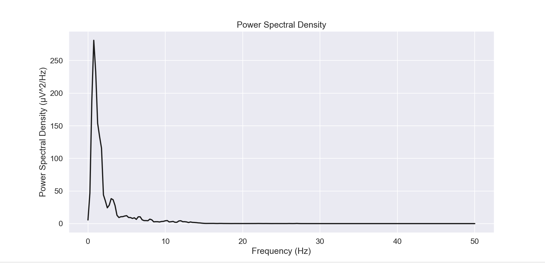

Applications

1. Clinical Diagnosis: Bandpower analysis is used to detect abnormalities such as epilepsy, sleep disorders, and brain injuries.
2. Cognitive Research: Analysis of EEG bandpowers provides insights into cognitive processes such as attention, memory, and learning.
3. Brain-Computer Interfaces (BCIs): Bandpower features are employed in BCIs for controlling external devices through neural signals.

Code

import numpy as np
import matplotlib.pyplot as plt
from scipy.signal import welch
import seaborn as sns
from scipy.integrate import simps
sns.set(font_scale=1.2)


# extract EEG from file
data_file = r"eeg-data.txt"
sfreq = 100
win = 4
# load EEG
eeg_data = np.loadtxt(data_file)
time = np.arange(eeg_data.size) / sfreq

# get psd using welch
frequencies, psd = welch(eeg_data, fs=sfreq, nperseg=sfreq*win)
freqres = frequencies[1] - frequencies[0]

freq_bands = {
    'Delta': (1, 4),
    'Theta': (4, 8),
    'Alpha': (8, 13),
    'Beta': (13, 30)
}

# get absolute bandpower
bandpower = {}
for band, (f_low, f_high) in freq_bands.items():
    idx_band = np.where((frequencies >= f_low) & (frequencies <= f_high))
    band_power = simps(psd[idx_band], dx=freqres)
    bandpower[band] = band_power

# get total power & relative bandpower
total_power = simps(psd, frequencies)
relative_bandpower = {band: power / total_power for band, power in bandpower.items()}
max_band = max(relative_bandpower, key=relative_bandpower.get)

print("Absolute Bandpower:")
for band, power in bandpower.items():
    print(f"{band}: {power:.4f} µV^2")

print("\nRelative Bandpower:")
for band, power in relative_bandpower.items():
    print(f"{band}: {power:.4f}")
print(f"\nThe frequency band with the highest relative bandpower is: {max_band.capitalize()}")
# Plot psd
plt.figure(figsize=(8, 4))
plt.plot(frequencies, psd, color='k', lw=2)
plt.xlabel('Frequency (Hz)')
plt.ylabel('Power Spectral Density (µV^2/Hz)')
plt.title('Power Spectral Density')
plt.grid(True)
plt.show()

Sources

1. Niedermeyer, E., & da Silva, F. L. (2004). Electroencephalography: Basic Principles, Clinical Applications, and Related Fields. Lippincott Williams & Wilkins.
2. Oken, B. S., & Chiappa, K. H. (1986). Short-term variability in EEG frequency analysis. Electroencephalography and Clinical Neurophysiology, 63(4), 353-367.
3. Cooley, J. W., & Tukey, J. W. (1965). An algorithm for the machine calculation of complex Fourier series. Mathematics of Computation, 19(90), 297-301.
4. Daubechies, I. (1990). The wavelet transform, time-frequency localization, and signal analysis. IEEE Transactions on Information Theory, 36(5), 961-1005.
5. Huang, N. E., Shen, Z., & Long, S. R. (1998). The empirical mode decomposition and the Hilbert spectrum for nonlinear and non-stationary time series analysis. Proceedings of the Royal Society of London. Series A: Mathematical, Physical and Engineering Sciences, 454(1971), 903-995.